Introduction
Ever wonder how you remember a song not just the tune, but how each note flows into the next? That’s exactly what Recurrent Neural Networks (RNNs) do for machines. Unlike traditional neural networks that treat inputs as isolated, RNNs retain a “memory” of previous data, making them ideal for tasks like language translation, speech recognition, and stock prediction. Think of it this way: a standard model forgets your name right after you say it. An RNN remembers your entire conversation from a month ago. But despite their strengths, standard RNNs face a major limitation that nearly made them obsolete. Want to build smart language or prediction models? Our AI Development services can help you create solutions that learn and adapt.

1. Understanding the Fundamentals of RNNs
What Are Recurrent Neural Networks?
RNNs are a type of neural network designed for sequential data.
Unlike traditional feedforward networks that treat inputs as independent, RNNs consider the order and context of input data.
They have a built-in memory mechanism.
RNNs retain information from previous time steps using a “hidden state” which is passed from one step to the next, allowing them to learn from past data.
RNNs excel in time-dependent tasks.
Their ability to model dependencies across time makes them ideal for natural language processing, speech recognition, video analysis, and time-series forecasting.
They operate recursively.
The same function is applied to each element of the sequence, ensuring that each input is processed with reference to the context established by prior inputs.
Key Characteristics That Define RNNs
Sequential Processing:
RNNs handle input data that comes in a sequence (e.g., text, audio, sensor data), maintaining continuity and temporal relationships.
Shared Parameters Across Time Steps:
RNNs reuse the same weights and biases for each time step, which simplifies the model and reduces the number of parameters.
Memory Retention:
RNNs carry a hidden state that stores context from previous inputs, making them capable of learning long-term and short-term dependencies.
Feedback Loops:
The output from the hidden layer is looped back as input for the next step, creating a feedback connection that gives the network its recurrent nature.
Difference Between RNNs and Feedforward Neural Networks
| Feature | RNN | Feedforward Neural Network |
|---|---|---|
| Data Handling | Sequential | Independent |
| Memory | Maintains hidden state | No memory |
| Input Flexibility | Handles variable-length input | Fixed-length input |
| Output | Dynamic, context-aware | Static, context-less |
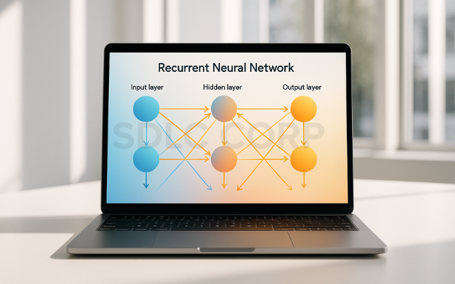
Core Components of RNN Architecture
Input Layer:
Takes one element of the input sequence at a time. For instance, each word in a sentence is processed one by one.
Hidden Layer:
Contains neurons that store the hidden state. It captures temporal dependencies using feedback loops. This is the part of the network that “remembers.”
Output Layer:
Produces a result at each time step. It could be the predicted next word, class label, or numerical value depending on the application.
Activation Function (commonly tanh or ReLU):
Introduces non-linearity to the model, allowing it to capture complex patterns.
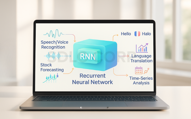
Real-World Scenarios Where RNNs Are Used
Text Prediction: Completing a sentence or generating next words in a chatbot.
Speech Recognition: Translating voice commands into text.
Stock Price Forecasting: Analyzing time-series data for future trends.
Machine Translation: Converting sentences from one language to another.
Handwriting Recognition: Predicting characters based on previous strokes.
Why RNNs Matter in AI & Deep Learning
They allow machines to understand sequences, just as humans do.
They are essential for tasks requiring context, such as answering questions or analyzing conversations.
They laid the groundwork for advanced sequence models like LSTMs, GRUs, and Transformers.
2. The Mathematics Behind RNNs
Forward Propagation in RNNs
Forward propagation is the core operation where the network computes outputs by passing inputs through neurons step-by-step, incorporating previous states.
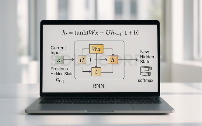
Mathematical Formula:
ht = tanh(Wxh · xt + Whh · ht-1 + bh)
yt = softmax(Why · ht + by)
Explanation of Terms:
- xt: Input at time step t
- ht-1: Previous hidden state
- Wxh, Whh, Why: Weight matrices
- bh, by: Bias vectors
- ht: New hidden state
- yt: Output at time step t
Backpropagation Through Time (BPTT)
Definition:
BPTT is the standard training algorithm for Recurrent Neural Networks (RNNs). It extends regular backpropagation by unrolling the RNN across time and computing gradients for each time step, enabling the model to learn temporal dependencies.
How BPTT Works:
- Unfold the RNN across time for each sequence input.
- Compute the loss at each time step:
Lt = -∑ yt · log(ŷt)
- Accumulate total loss:
Ltotal = ∑ Lt
- Compute gradients of loss with respect to weights:
∂L/∂W = ∑ ∂L/∂ht · ∂ht/∂W
- Update weights using gradient descent.
Key Issues in BPTT:
- Vanishing gradients: Hinders learning long-term dependencies.
- Exploding gradients: Causes unstable training.
- Solutions: Use LSTM/GRU, gradient clipping, adaptive optimizers.
Activation Functions for RNNs
Activation functions introduce non-linearity into neural networks and are essential for allowing RNNs to learn complex temporal patterns. In RNNs, they are typically applied to the hidden state and sometimes the output layer.
Common Activation Functions in RNNs:
- Tanh (Hyperbolic Tangent)
tanh(x) = (e^x - e^(-x)) / (e^x + e^(-x))
Outputs range from -1 to 1. Helps preserve gradient flow. Commonly used in standard RNN hidden states.
- Sigmoid (Logistic Function)
σ(x) = 1 / (1 + e^(-x))
Outputs range from 0 to 1. Used in LSTM and GRU gates to control information flow.
- ReLU (Rectified Linear Unit)
ReLU(x) = max(0, x)
Helps reduce vanishing gradients. Less common in traditional RNNs, but used in modern architectures.
3. Common Challenges with RNNs
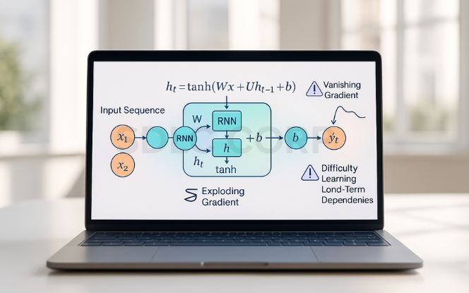
The Vanishing Gradient Problem
One of the most well-known issues in training RNNs is the vanishing gradient problem. During backpropagation through time (BPTT), gradients of the loss function can shrink exponentially as they are passed backward through many time steps.
As a result, weights stop updating effectively, especially for earlier layers.
This makes it hard for standard RNNs to learn long-term dependencies or retain useful context across long sequences.
Exploding Gradient Problem
The opposite of vanishing gradients, exploding gradients occur when the gradients become excessively large, causing the weights to overshoot during updates.
This leads to unstable training and sometimes NaN (Not a Number) losses.
It usually happens when the weight matrices in the recurrent loop have large eigenvalues.
Solution: Gradient clipping is a common technique to prevent this issue by limiting the size of the gradient during training.
Difficulty in Capturing Long-Term Dependencies
Standard RNNs are inherently weak at capturing long-range dependencies in sequential data due to memory fading over time.
Tasks like machine translation or document summarization, where early context is crucial, suffer with basic RNNs.
LSTM and GRU architectures were introduced specifically to resolve this limitation.
Sequential Computation and Slow Training
RNNs process input one step at a time, which limits their ability to leverage parallelization during training.
Unlike transformers or CNNs, which can process data in parallel, RNNs must complete each time step sequentially.
This leads to longer training times and higher computational costs for large datasets.
Limited Scalability for Long Sequences
RNNs tend to perform poorly as the length of input sequences increases. Memory consumption and training complexity rise with sequence length.
BPTT must store all intermediate states across time, which uses up RAM.
In practice, many models truncate sequences or limit the number of backpropagated steps, compromising accuracy.
Overfitting on Small Datasets
Due to their high model complexity, RNNs are prone to overfitting, especially when used on small or noisy datasets.
They may learn temporal noise rather than general patterns.
Regularization methods like dropout, early stopping, and weight decay are often used.
Interpretability and Debugging
Unlike simpler models, RNNs operate as black boxes, making it difficult to understand:
Which time steps influenced the output most
Why certain predictions were made
What information was forgotten or remembered
Tools like attention mechanisms and saliency maps help improve transparency, but interpretability remains a challenge.
4. Advanced RNN Architectures

Long Short-Term Memory (LSTM)
LSTM networks are designed to solve the vanishing gradient problem and effectively capture long-term dependencies.
Key Components:
- Cell state (Ct): Long-term memory flow
- Input gate: Controls input writing
- Forget gate: Controls memory erasure
- Output gate: Controls output extraction
LSTM Equations:
f_t = σ(W_f · [h_(t-1), x_t] + b_f)
i_t = σ(W_i · [h_(t-1), x_t] + b_i)
C̃_t = tanh(W_C · [h_(t-1), x_t] + b_C)
C_t = f_t * C_(t-1) + i_t * C̃_t
o_t = σ(W_o · [h_(t-1), x_t] + b_o)
h_t = o_t * tanh(C_t)
Gated Recurrent Unit (GRU)
GRU simplifies LSTM by combining input and forget gates into one and using fewer parameters.
Key Features:
- Faster training
- Efficient for real-time and mobile apps
GRU Equations:
z_t = σ(W_z · [h_(t-1), x_t])
r_t = σ(W_r · [h_(t-1), x_t])
h̃_t = tanh(W · [r_t * h_(t-1), x_t])
h_t = (1 - z_t) * h_(t-1) + z_t * h̃_t
Bidirectional RNN (BiRNN)
Bidirectional Recurrent Neural Networks extend the standard RNN by processing input sequences in both forward and backward directions. Instead of relying solely on past context, the model has access to future context as well.
In this architecture, two separate hidden layers are used:
One processes the sequence from beginning to end.
The other processes it from end to beginning.
The outputs from both directions are then combined, providing richer contextual information at every time step.
Advantages:
Enhances performance on tasks where full sequence context improves accuracy.
Deep or Stacked RNN
Stacked RNNs consist of multiple RNN layers, allowing the model to learn complex temporal hierarchies.
Benefits:
- Improved abstraction of sequential data
- Useful for video and long-text modeling
Attention-Enhanced RNNs
Attention mechanisms help RNNs focus on important parts of a sequence, improving performance in complex tasks.
Benefits:
- Dynamic focus on relevant time steps
- Excellent for machine translation and summarization
Recursive Neural Networks (Tree-RNNs)
Recursive Neural Networks (not to be confused with recurrent) apply the same set of weights in a tree-structured fashion rather than linear sequences.
Use Cases:
Parsing and sentiment analysis in hierarchical structures like sentences or code trees.
Hierarchical RNNs (HRNNs)
Hierarchical RNNs break down long sequences into sub-units and process each level with its own RNN.
Applications:
Document-level classification
Hierarchical language generation
Recurrent Highway Networks (RHNs)
Recurrent Highway Networks are a deeper and more expressive variant of RNNs, combining ideas from residual connections and highway networks. They allow for the construction of deep recurrent transitions between time steps while preserving gradient flow.
Key features:
Gated transformation and carry mechanisms control how much information is transformed versus passed through unchanged.
Helps train deeper RNNs without suffering from vanishing gradients.
Benefits:
Enables modeling of more complex temporal dynamics.
Improves training stability and expressiveness over standard RNNs.
5. Real-World Applications of RNNs
Natural Language Processing (NLP)
RNNs are foundational to many language-based AI tasks, especially when input and output sequences vary in length or structure.
Key Use Cases:
Text generation: Auto-writing tools, email suggestions, and storytelling AI (e.g., GPT-style models)
Machine translation: Converting one language to another using sequence-to-sequence models
Sentiment analysis: Detecting positive, negative, or neutral tones in customer reviews, tweets, or surveys
Named Entity Recognition (NER): Identifying people, places, dates, etc., in text streams
Speech Recognition and Audio Processing
RNNs shine in speech-to-text and audio understanding tasks due to their sequence alignment capabilities.
Key Use Cases:
Voice assistants: Siri, Alexa, and Google Assistant use RNNs (and variants) to transcribe spoken commands.
Real-time transcription: Tools like Otter.ai and Zoom captions.
Speaker identification: Recognizing who is speaking in a recording.
Time-Series Forecasting
RNNs can model and predict trends in time-based data, making them ideal for industries that rely on forecasting.
Key Use Cases:
Stock price prediction: Forecasting financial markets using historical patterns
Energy consumption forecasting: For smart grids and utility planning
Weather prediction: Predicting temperatures, rainfall, or natural disasters
Sales and demand forecasting: Inventory management and trend analysis in eCommerce
Healthcare and Medical Diagnostics
With large datasets of patient records and monitoring data, RNNs can support life-saving decision systems.
Key Use Cases:
ECG signal analysis: Detecting irregularities or predicting heart anomalies
Patient health monitoring: Predicting critical events based on time-stamped data
Electronic health record (EHR) analysis: Mining sequential data from patient history for early diagnosis
Video Processing and Captioning
RNNs, often combined with CNNs or transformers, help understand and describe temporal sequences in video frames.
Key Use Cases:
Video captioning: Automatically describing video content frame-by-frame
Activity recognition: Detecting human actions like walking, running, jumping in surveillance or sports
Gesture control: Understanding hand movements for gaming or virtual interfaces
Anomaly Detection in Cybersecurity
RNNs can monitor logs and traffic over time to detect abnormal or malicious patterns.
Key Use Cases:
Intrusion detection: Spotting unexpected access or network behaviors
Fraud detection: Analyzing sequences of user actions or transactions
System log analysis: Identifying deviations in operational sequences
6. Implementing RNNs in Practice
Data Preprocessing for RNNs
RNNs require sequential input data, so careful preprocessing is essential.
Key Steps:
Tokenization: For text, split sentences into words or characters.
Normalization: Convert inputs to lowercase, remove punctuation, or scale numerical values.
Padding/Truncation: Ensure sequences are of equal length using padding (e.g., with zeros).
Reshaping: Input shape should be (samples, time steps, features).
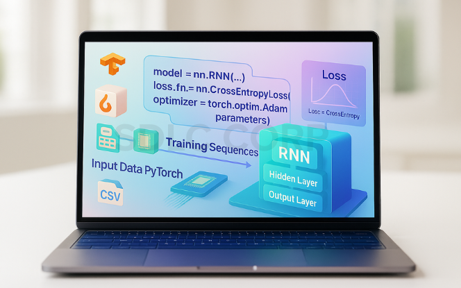
Building a Basic RNN Model
You can build a simple RNN using Keras in just a few lines:
from keras.models import Sequential
from keras.layers import SimpleRNN, Dense

model = Sequential()
model.add(SimpleRNN(units=64, input_shape=(timesteps, features)))
model.add(Dense(units=1, activation='sigmoid'))
model.compile(optimizer='adam', loss='binary_crossentropy',
metrics=['accuracy'])
Choosing the Right RNN Variant
SimpleRNN: Best for basic, short-sequence problems
LSTM: Best for long-term memory and time-series data
GRU: Faster training than LSTM, with competitive performance
Bidirectional RNN: When both past and future context matter
Training the RNN
Use the .fit() function to train your RNN:
history = model.fit(X_train, y_train, epochs=10, batch_size=32, validation_split=0.2)
- ✔ Use Adam or RMSprop optimizers
- ✔ Add Dropout layers to reduce overfitting
- ✔ Monitor metrics like accuracy, loss, or MSE
Evaluating and Monitoring RNN Performance
Effective implementation of RNNs goes beyond model definition and training it requires careful evaluation and ongoing monitoring to ensure the model is learning as expected and generalizing well.
Common Evaluation Metrics
1. Classification Tasks
Accuracy:
Measures the proportion of correct predictions over total predictions.
Cross-Entropy Loss:
Evaluates the divergence between predicted and actual probability distributions.
Lower values indicate better performance.
2. Regression Tasks
Mean Squared Error (MSE):
Penalizes larger errors more than smaller ones.
Ideal for capturing sensitivity to large deviations.
Mean Absolute Error (MAE):
Measures the average absolute differences between predicted and actual values.
More interpretable for real-world values.
3. Language Models
Perplexity:
Evaluates how well the model predicts a sequence of words.
A lower perplexity score indicates better predictive performance.
Visualization Techniques
Visual feedback is essential for detecting issues like overfitting, underfitting, or instability during training.
1 Helpful Visual Tools:
Learning Curves:
Plot training and validation loss/accuracy over epochs.
➤ Helps identify early stopping points or overfitting.
Confusion Matrix:
For classification problems, it shows which classes are being misclassified.
➤ Ideal for multi-class model diagnosis.
Loss Surface Trends:
Tracks how noisy or stable your loss function appears across training.
➤ A spiky curve may indicate poor optimization or bad initialization.
Monitoring Tools
These tools help you log, compare, and debug experiments efficiently:
1. Tensor Board (for TensorFlow/Keras)
Visualize training/validation loss, accuracy, and histograms
Track computational graphs and embeddings
Analyze performance across time and layers
2. Weights & Biases (wandb)
Real-time dashboard for metrics, gradients, and losses
Hyperparameter sweep and version control
Team collaboration and model versioning
Works with PyTorch, TensorFlow, Keras, and more

Conclusion
Recurrent Neural Networks (RNNs) offer powerful capabilities for processing sequential and time-dependent data. As their architectures evolve, they remain essential in solving complex problems across industries. If you’re looking to integrate RNNs into your products or workflows, our team provides end-to-end AI development services from model design to deployment to help you build intelligent, context-aware solutions.
FAQs
1. What is the main difference between RNNs and traditional neural networks?
RNNs have loops that allow them to retain memory across time steps, making them ideal for sequential data. Traditional neural networks treat each input independently without context.
2. Why do RNNs struggle with long-term dependencies?
Because of the vanishing gradient problem. During training, gradients shrink as they backpropagate through time, making it difficult to learn patterns from earlier in the sequence.
3. When should I use LSTM or GRU instead of a vanilla RNN?
Use LSTM or GRU when your task involves long-term dependencies or complex sequence data. They include gating mechanisms that help manage memory and mitigate gradient issues.
4. Are RNNs still relevant with the rise of Transformers?
Yes, while Transformers dominate NLP tasks, RNNs are still effective for real-time applications, smaller datasets, and tasks requiring compact models with temporal awareness.
5. What are common real-world applications of RNNs?
RNNs are used in natural language processing, speech recognition, stock market prediction, weather forecasting, music generation, and medical time series analysis.
6. What tools should I use to implement RNNs?
Popular frameworks include TensorFlow (Keras), PyTorch, and JAX. Each offers excellent support for RNN layers, data preprocessing, and model training workflows.